3. Discretization Approach

Nalu supports two discretizations: control volume finite element and (CVFEM) edge-based vertex centered (EBVC). Each are finite volume forumations and each solve for the primitives are are each considered vertex-based schemes. Considerable testing has provided a set of general rules as to which scheme is optimal. In general, all equations and boundary conditions support either equation discretization with exception of the solid stress equation which has only been implemented for the CVFEM technique.

For generalized unstructured meshes that have poor quality, CVFEM has been shown to excell in accuracy and robustness. This is mostly due to the inherent accuracy limitation for the non-orthogonal correction terms that appear in the diffusion term and pressure stabilization for the EBVC scheme. For generalized unstructured meshes of decent quality, either scheme is ideal. Finally, for highly structured meshes with substantail aspect ratios, the edge-based scheme is ideal.

In general, the edge-based scheme is at least two times faster per iteration than the element-based scheme. For some classes of flows, it can be up to four times faster. However, due to the lagged coupling between the projected nodal gradient equation and the dofs, on meshes with high non-orthogonality, nonlinear residual convergence can be delayed.

3.1. CVFEM Dual Mesh

The classic low Mach algorithm uses the finite volume technique known as the control volume finite element method, see Schneider, [SR87], or Domino, [Dom06]. Control volumes (the mesh dual) are constructed about the nodes, shown in Figure Fig. 3.1 (upper left). Each element contains a set of sub-faces that define control-volume surfaces. The sub-faces consist of line segments (2D) or surfaces (3D). The 2D segments are connected between the element centroid and the edge centroids. The 3D surfaces (not shown here) are connected between the element centroid, the element face centroids, and the edge centroids. Integration points also exist within the sub-control volume centroids.

Recent work by Domino, [Dom14], has provided a proof-of-concept higher order CVFEM implementation whereby the linear basis and dual mesh definition is extended to higher order. The current code base supports the usage of P=2 elements (quadratic) for both 2D and 3D quad/hex topologies. This method has been formally demonstrated to be third-order spatially accurate and second-order in-time accurate. General polynomial promotion has been deployed in the higher order github branch. Figure Fig. 3.1 illustrates a general polynomial promotion from P=1 to P=6 and demonstrated spectral convergence using the method of manufactured solutions in Figure Fig. 3.2.

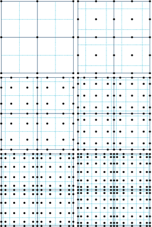
Fig. 3.1 Polynomial promotion for a canonical CVFEM quad element patch from \(P=1\) to \(P=6\).

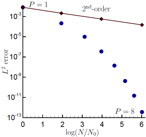
Fig. 3.2 A recent spectral convergence plot using the Method of Manufactured Solutions for \(P=1\) through \(P=8\).

When using CVFEM, the discretized equations described in this manual are evaluated at either subcontrol-surface integration points (terms that have been integrated by parts) or at the subcontrol volume (time and source terms). Interpolation within the element is obtained by the standard elemental basis functions,

(3.1)\[{\phi_{ip} = \sum N^{ip}_k \phi_k.}\]

where the index \(k\) represents a loop over all nodes in the element.

Gradients at the subcontrol volume surfaces are obtained by taking the derivative of Eq. (3.1), to obtain,

(3.2)\[\frac{\partial \phi_{ip}}{\partial x_j} = \sum \frac{\partial N^{ip}_{j,k}} {\partial x_j} \phi_k.\]

The usage of the CVFEM methods results in the canonical 27-point stencil for a structured hexahedral mesh.

3.2. Edge-Based Discretization

In the edge-based discretization, the dual mesh defined in the CVFEM method is used to pre-process both dual mesh nodal volumes (needed in source and time terms) and edge-based area vectors (required for integrated-by-parts quantities, e.g., advection and diffusion terms).

Fig. 3.3 A control volume centered about a finite-element node in a collection of 2-D quadrilateral elements (from [Dom06].)

Consider Figure Fig. 3.3, which is the original set of CVFEM dual mesh quadrature points shown above in Figure Fig. 3.1. Specifically, there are four subcontrol volumes about node 5 that contribute to the nodal volume dual mesh. In an edge-based scheme, the time and source terms use single point quadrature by assembling these four subcontrol volume contributions (eight in 3D) into one single nodal volume. In most cases, source terms may include gradients that are obtained by using the larger element-based stencil.

The same reduction of gauss points is realized for the area vector. Consider the edge between nodes 5 and 6. In the full CVFEM approach, subcontrol surfaces within the top element (5,6,9,8) and bottom element (2,3,6,5) are reduced to a single area vector at the edge midpoint of nodes 5 and 6. Therefore, advection and diffusion is now done in a manner very consistent with a cell centered scheme, i.e., classic “left”/“right” states.

The consolidation of time and source terms to nodal locations along with advection and diffusion at the edge mid-point results in a canonical five-point stencil in 2D and seven in 3D. Note the ability to handle hybrid meshes is readily peformed one nodal volume and edge area are pre-processed. Edges and nodes are the sole topology that are iterated, thus making this scheme highly efficient, although inherantly limited to second order spatial order of accuracy.

In general, the edge-based scheme is second order spatially accurate. Formal verification has been done to evaluate the accuracy of the EBVC relative to other implemented methods (Domino, [Dom14]). The edge-based scheme, which is based on dual mesh post-processing, represents a commonly used finite volume method in gas dynamics applications. The method also lends itself to psuedo-higher order methodologies by the blending of extrapolated values using the projected nodal gradient and gauss point values (as does CVFEM). This provides a fourth order accurate diffusion and advection operator on a structured mesh.

The use of a consistent mass matrix is less apparent in edge-based schemes. However, if desired, the full element-based stencil can be used by iterating elements and assembling to the nodes.

The advantage of edge-based schemes over cell centered schemes is that the scheme naturally allows for a mixed elemental discretization. Projected nodal gradients can be element- or edge-based. LES filters and nodal gradients can also exploit the inherant elemental basis that exists in the pure CVFEM approach. In our experience, the optimal scheme on high quality meshes uses the CVFEM for the continuity solve and EBVC discretization for all other equations. This combination allows for the full CVFEM diffusion operator for the pressure Poisson equation and the EBVC approach for equations where inverse Reynolds scaling reduces the importance of the diffusion operator. This scheme can be activated by the use of the use_edges: yes Realm line command in combination of the LowMachEOM system line command, element_continuity_eqs: yes.

3.3. Projected Nodal Gradients

In the edge or element-based algorithm, projected nodal gradients are commonplace. Projected nodal gradients are used in the fourth order pressure stabilization terms, higher order upwind methods, discontinuity capturing operators (DCO) and turbulence source terms. For an edge-based scheme, they are also used in the diffusion term when non-orthogonality of the mesh is noted.

There are many procedures for determining the projected nodal gradient ranging from element-based schemes to edge-based approached. In general, the projected nodal gradient is viewed as an \(L_2\) minimization between the discontinuous Gauss-point value and the continuous nodal value. The projected nodal gradient, in an \(L_2\) sence is given by,

(3.3)\[\int w G_j \phi {dV} = \int \frac{\partial \phi}{\partial x_j}{dV}.\]

Using integration-by-parts and a piece-wise constant test function, the above equation is written as,

(3.4)\[\int w_I G_j \phi {dV} = \int \phi_{ip} n_j {dS}.\]

For a lumped L2 projected nodal gradient, the approach is based on a Green-Gauss integration,

(3.5)\[G_j \phi = \frac{\int \phi_{ip} A_j}{dV}.\]

In the above lumped mass matrix approach, the value at the integration point can either be based on the CVFEM dual mesh evaluated at the subcontrol surface, i.e., the line command option, element or the edge, which evaluates the term at the edge midpoint using the assemble edge area vector. In all cases, the lumped mass matrix approach is strickly second order accurate. When running higher order CVFEM, a consistent mass matrix appraoch is required to maintain design order of the overall discretization. This is strickly due to the pressure stabilization whose accuracy can be affected by the form of the projected nodal gradient (see the Nalu theory manual or a variety of SNL-based publications).

In the description that follows, \(\bar{G_j \phi}\) represent the average nodal gradient evaluated at the integration point of interest.

The choice of projected nodal gradients is specified in the input file for each dof. Keywords element or edge are used to define the form of the projection. The forms of the projected nodal gradients is arbitrary relative to the choosed underlying discretization. For strongly non-orthogonal meshes, it is recommended to use an element-based projected nodal gradient for the continuity equation when the EBVC method is in use. In some limited cases, e.g., pressure, mixture fraction and enthalpy, the manage-png line command can be used to solve the simple linear system for the consistent mass matrix.

3.4. Time and Source Terms

Time and source terms also volumetric contributions and also use the dual nodal volume. In both discretization approaches, this assembly is achieved as a simple nodal loop. In some cases, e.g., the \(k_{sgs}\) partial differential equation, the source term can use projected nodal gradients.

\[\int \frac{\partial \rho \phi }{\partial t} dV = \int S_{\phi}dV\]

3.5. Diffusion

As already noted, for the CVFEM method, the diffusion term at the subcontrol surface integration points use the the elemental shape functions and derivatives. For the standard diffusion term, and using Eq. (3.2), the CVFEM diffusion operator contribution at a given integration point (here simply demonstrated for a 2D edge with prescribed area vector) is as follows,

\[-\int \Gamma \frac{\partial \phi}{\partial x_j} A_j = - \Gamma_{ip} \left[ \left(\frac{\partial N^{ip}_0} {\partial x} \phi_0 + \frac{\partial N^{ip}_1} {\partial x} \phi_1 \right) A_x + \left(\frac{\partial N^{ip}_0} {\partial y} \phi_0 + \frac{\partial N^{ip}_1} {\partial y} \phi_1 \right) A_y \right]\]

Standard Gauss point locations at the subcontrol surfaces can be shifted to the edge-midpoints for a more stable (monotonic) diffusion operator that is better conditioned for high aspect ratio meshes.

For the edge-based diffusion operator, special care is noted as there is no ability to use the elemental basis to define the diffusion operator. As with cell-centered schemes, non-orthogonal contributions for the diffusion operator arise due to a difference in direction between the assembled edge area vector and the distance vector between nodes on an edge. On skewed meshes, this non-orthogonality can not be ignored.

Following the work of Jasek, [Jas96], the over-relaxed approach is used. The form of any gradient for direction \(j\) for field \(\phi\) is

(3.6)\[\frac{\partial \phi}{\partial x_j}_{ip} = \bar{G_j\phi} + \left[ \left(\phi_R - \phi_L \right) - \bar{G_l\phi}dx_l \right] \frac{A_j}{A_k dx_k}.\]

In the above expression, we are iterating edges with a Left node \(L\) and Right node \(R\) along with edge-area vector, \(A_j\). The \(\bar{G_j \phi}\) is simple averaging of the left and right nodes to the edge midpoint. In general, a standard edge-based diffusion term is written as,

\[\begin{split}-\int \Gamma \frac{\partial \phi}{\partial x_j} A_j &= - \Gamma_{ip} \left[ \left(\bar{G_x \phi}A_x + \bar{G_y \phi}A_y \right) + \left( \phi_R - \phi_L \right) \frac{A_x A_x + A_y A_y}{A_x dx_x + A_y dx_y} \right. \\ &- \left. \left( \bar{G_x \phi}dx_x + \bar{G_y \phi}dx_y \right) \frac{A_x A_x + A_y A_y} {A_x dx_x + A_y dx_y} \right].\end{split}\]

3.5.1. Momentum Stress

The viscous stress tensor, \(\tau_{ij}\) is formed based on the standard gradients defined above for either the edge or element-based discretization. The viscous force for component \(i\) is given by,

\[-\int \tau_{ij} A_j = -\int \mu_{ip}\left( \frac{\partial u_i}{\partial x_j} + \frac{\partial u_j}{\partial x_i} \right) A_j.\]

For example, the x and y-component of viscous force is given by,

\[\begin{split}F_x &= - \mu_{ip} \left( \frac{\partial u_x}{ \partial x}A_x + \frac{\partial u_x}{\partial y}A_y \right ) - \mu_{ip} \left( \frac{\partial u_x}{ \partial x}A_x + \frac{\partial u_y}{ \partial x}A_y \right), \\ F_y &= - \mu_{ip} \left( \frac{\partial u_y}{ \partial x}A_x + \frac{\partial u_y}{\partial y}A_y \right ) - \mu_{ip} \left( \frac{\partial u_x}{ \partial y}A_x + \frac{\partial u_y}{ \partial y}A_y \right).\end{split}\]

Note that the first part of the viscous stress is simply the standard diffusion term. Note that the so-called non-solonoidal viscous stress contribution is frequently written in terms of projected nodal gradients. However, for CVFEM this procedure is rarely used given the elemental basis definition. As such, the use of shape function derivatives is clear.

The viscous stress contribution at an integration point for CVFEM (again using the 2D example with variable area vector) can be written as,

\[\begin{split}F_x &= - \Gamma_{ip} \left[ \left(\frac{\partial N^{ip}_0} {\partial x} {u_x}_0 + \frac{\partial N^{ip}_1} {\partial x} {u_x}_1 \right) A_x + \left(\frac{\partial N^{ip}_0} {\partial y} {u_x}_0 + \frac{\partial N^{ip}_1} {\partial y} {u_x}_1 \right) A_y \right. \\ &+ \left. \left(\frac{\partial N^{ip}_0} {\partial x} {u_x}_0 + \frac{\partial N^{ip}_1} {\partial x} {u_x}_1 \right) A_x + \left(\frac{\partial N^{ip}_0} {\partial y} {u_y}_0 + \frac{\partial N^{ip}_1} {\partial x} {u_y}_1 \right) A_y \right], \\ F_y &= - \Gamma_{ip} \left[ \left(\frac{\partial N^{ip}_0} {\partial x} {u_y}_0 + \frac{\partial N^{ip}_1} {\partial x} {u_y}_1 \right) A_x + \left(\frac{\partial N^{ip}_0} {\partial y} {u_y}_0 + \frac{\partial N^{ip}_1} {\partial y} {u_y}_1 \right) A_y \right. \\ &+ \left. \left(\frac{\partial N^{ip}_0} {\partial y} {u_x}_0 + \frac{\partial N^{ip}_1} {\partial y} {u_x}_1 \right) A_x + \left(\frac{\partial N^{ip}_0} {\partial y} {u_y}_0 + \frac{\partial N^{ip}_1} {\partial x} {u_y}_1 \right) A_y \right].\end{split}\]

For the edge-based diffusion operator, the value of \(\phi\) is substituted for the component of velocity, \(u_i\) in the Eq. (3.6).

\[\frac{\partial u_i}{\partial x_j}_{ip} = \bar{G_j u_i} + \left[ \left({u_i}_R - {u_i}_L \right) - \bar{G_l u_i}dx_l \right] \frac{A_j}{A_k dx_k}.\]

Common approaches in the cell-centered community are to use the projected nodal gradients for the \(\frac{\partial u_j}{\partial x_i}\) stress component. However, in Nalu, the above form of equation is used.

Substituting the relations of the velocity gradients for the x and y-componnet of force above provides the following expression used for the viscous stress contribution:

\[\begin{split}F_x &= - \mu_{ip} \left[ \left(\bar{G_x u_x}A_x + \bar{G_y u_x}A_y \right) + \left( {u_x}_R - {u_x}_L \right) \frac{A_x A_x + A_y A_y}{A_x dx + A_y dy} \right. \\ &- \left. \left( \bar{G_x u_x}dx + \bar{G_y u_x}dy \right) \frac{A_x A_x + A_y A_y} {A_x dx + A_y dy} \right] \\ &- \mu_{ip} \left[ \bar{G_x u_x}A_x + \bar{G_x u_y}A_y + \left({u_x}_R - {u_x}_L\right) \frac{A_x A_x} {A_x dx + A_y dy} \right. \\ &+ \left. \left({u_y}_R - {u_y}_L\right) \frac{A_x A_y} {A_x dx + A_y dy} \right. \\ &- \left. \left( \bar{G_x u_x}dx + \bar{G_y u_x}dy \right) \frac{A_x A_x} {A_x dx + A_y dy} \right. \\ &- \left. \left( \bar{G_x u_y}dx + \bar{G_y u_y}dy \right) \frac{A_x A_y} {A_x dx + A_y dy} \right],\end{split}\]

\[\begin{split}F_y &= - \mu_{ip} \left[ \left(\bar{G_x u_y}A_x + \bar{G_y u_y}A_y \right) + \left( {u_y}_R - {u_y}_L \right) \frac{A_x A_x + A_y A_y}{A_x dx + A_y dy} \right. \\ &- \left. \left( \bar{G_x u_y}dx + \bar{G_y u_y}dy \right) \frac{A_x A_x + A_y A_y} {A_x dx + A_y dy} \right] \\ &- \mu_{ip} \left[ \bar{G_y u_x}A_x + \bar{G_y u_y}A_y + \left({u_y}_R - {u_y}_L\right) \frac{A_y A_y} {A_x dx + A_y dy} \right. \\ &+ \left. \left({u_x}_R - {u_x}_L\right) \frac{A_y A_x} {A_x dx + A_y dy} \right. \\ &- \left. \left( \bar{G_x u_y]}dx + \bar{G_y u_y}dy \right) \frac{A_y A_y} {A_x dx + A_y dy} \right. \\ &- \left. \left( \bar{G_x u_x}dx + \bar{G_y u_x}dy \right) \frac{A_y A_x} {A_x dx + A_y dy} \right],\end{split}\]

where above, the first \([]\) and second \([]\) represent the \(\frac{\partial u_i}{\partial x_j}A_j\) and \(\frac{\partial u_j}{\partial x_i}A_j\) contributions, respectively.

One can use this expression to recognize the ideal LHS sensitivities for row and columns for component \(u_i\).